Database Architecture Patterns for High-Scale Enterprise Applications

The Database Scaling Cliff

There’s a pattern I’ve seen repeatedly in growing enterprises: an application hums along for years, then hits a wall. Queries that took milliseconds now take seconds. Writes queue. Connections exhaust. The database that served the business faithfully becomes the bottleneck that threatens it.

This isn’t a failure of technology. It’s a failure of architecture. Early database decisions—made when the dataset was small and the team was building quickly—create constraints that become visible only at scale. By then, the cost of changing course is enormous.

The organisations that scale gracefully made different architectural choices early. Not necessarily more complex choices—often simpler ones with clearer boundaries. They understood that database architecture isn’t about selecting the best technology; it’s about matching data patterns to storage patterns and planning for growth that hasn’t happened yet.

This post explores the patterns that enable that graceful scaling.

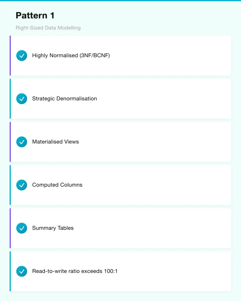
Pattern 1: Right-Sized Data Modelling

Most database performance problems trace back to data modelling decisions made in the first weeks of development.

The Normalisation Trade-off

Relational database theory teaches normalisation: eliminate redundancy, store each fact once, join at query time. This is correct for data integrity. It’s often wrong for performance.

Highly Normalised (3NF/BCNF):

-- To get customer order details:
SELECT c.name, o.order_date, p.product_name, oi.quantity
FROM customers c
JOIN orders o ON c.customer_id = o.customer_id
JOIN order_items oi ON o.order_id = oi.order_id
JOIN products p ON oi.product_id = p.product_id
WHERE c.customer_id = 12345;

Four table joins for a common query. At scale, joins become expensive—especially when tables span billions of rows.

Strategic Denormalisation:

-- Denormalised for read performance
SELECT customer_name, order_date, product_name, quantity
FROM order_details_view
WHERE customer_id = 12345;

Denormalisation pre-computes join results, trading write complexity for read simplicity.

When to Denormalise

Denormalise when:

• Read-to-write ratio exceeds 100:1
• Join tables exceed millions of rows
• Query patterns are well-known and stable
• Data freshness requirements allow for async updates

Keep normalised when:

• Write consistency is paramount
• Query patterns are unpredictable
• Data volumes are manageable
• Referential integrity is business-critical

Practical Denormalisation Strategies

Materialised Views Pre-computed query results that refresh periodically:

CREATE MATERIALIZED VIEW order_summary AS
SELECT
    customer_id,
    customer_name,
    COUNT(*) as order_count,
    SUM(total) as lifetime_value
FROM customers c
JOIN orders o USING (customer_id)
GROUP BY customer_id, customer_name;

-- Refresh on schedule
REFRESH MATERIALIZED VIEW CONCURRENTLY order_summary;

Computed Columns Store derived values alongside source data:

ALTER TABLE orders
ADD COLUMN item_count INTEGER GENERATED ALWAYS AS (
    SELECT COUNT(*) FROM order_items WHERE order_id = orders.order_id
) STORED;

Summary Tables Aggregate data for reporting workloads:

-- Maintained by triggers or scheduled jobs
CREATE TABLE daily_sales_summary (
    date DATE,
    region VARCHAR(50),
    product_category VARCHAR(50),
    total_sales DECIMAL(12,2),
    order_count INTEGER,
    PRIMARY KEY (date, region, product_category)
);

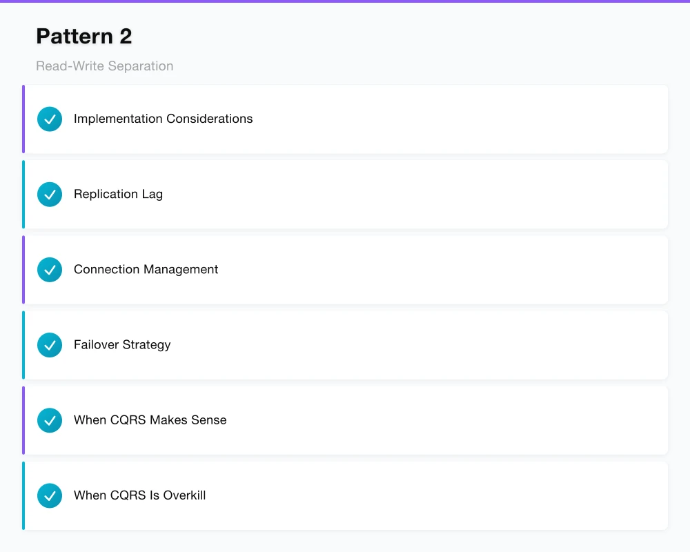
Pattern 2: Read-Write Separation

High-scale applications have different read and write characteristics. Treating them identically wastes capacity.

Primary-Replica Architecture

Route writes to the primary database; distribute reads across replicas:

[Application]
     |
     +---> [Write: Primary Database]
     |            |
     |            +---> [Replication] ---> [Replica 1]
     |                                ---> [Replica 2]
     |                                ---> [Replica 3]
     |
     +---> [Read: Load Balancer] ---> [Replicas]

Implementation Considerations:

Replication Lag Replicas may lag behind the primary by milliseconds to seconds. Applications must handle:

• Read-after-write consistency (read own writes from primary)
• Eventual consistency for non-critical reads
• Monitoring and alerting on lag thresholds

Connection Management Separate connection pools for read and write operations:

# Application connection management
class DatabasePool:
    def __init__(self):
        self.write_pool = create_pool(primary_host, size=50)
        self.read_pool = create_pool(replica_hosts, size=200)

![Pattern 2: Read-Write Separation Infographic](/images/database-architecture-patterns-high-scale-enterprise-applications-pattern-2-read-write-separation.webp)

    def get_write_connection(self):
        return self.write_pool.acquire()

    def get_read_connection(self):
        return self.read_pool.acquire()

Failover Strategy When the primary fails:

1. Detect failure (health checks, monitoring)
2. Promote replica to primary
3. Reconfigure other replicas to follow new primary
4. Update connection routing
5. Restore redundancy by adding new replica

Managed databases (RDS, Cloud SQL, Azure SQL) handle this automatically. Self-managed deployments require tooling (Patroni for PostgreSQL, Orchestrator for MySQL).

CQRS: Command Query Responsibility Segregation

Take read-write separation further by using different data stores for commands (writes) and queries (reads):

[Commands] --> [Event Store] --> [Event Processor] --> [Query Store]
                                                            |
[Queries] <------------------------------------------------+

The command store optimises for write consistency; the query store optimises for read performance. Event processing synchronises them asynchronously.

When CQRS Makes Sense:

• Wildly different read and write patterns
• Read performance requirements that relational queries can’t meet
• Complex domain logic benefiting from event sourcing
• Teams comfortable with eventual consistency

When CQRS Is Overkill:

• Read and write patterns are similar
• Team unfamiliar with event-driven architecture
• Strong consistency is non-negotiable
• Operational complexity isn’t justified

Pattern 3: Horizontal Partitioning (Sharding)

When a single database instance can’t handle your data volume or write throughput, distribute data across multiple instances.

Sharding Strategies

Range-Based Sharding Partition by value ranges:

Shard 1: customer_id 1-1,000,000
Shard 2: customer_id 1,000,001-2,000,000
Shard 3: customer_id 2,000,001-3,000,000

Advantages: Range queries stay on single shard, easy to understand Disadvantages: Uneven distribution if ranges vary in activity

Hash-Based Sharding Partition by hash function:

shard = hash(customer_id) % num_shards

Advantages: Even distribution, no hot spots Disadvantages: Range queries span all shards

Directory-Based Sharding Maintain a lookup table mapping keys to shards:

-- Lookup table
CREATE TABLE shard_directory (
    customer_id INTEGER PRIMARY KEY,
    shard_id INTEGER
);

Advantages: Flexible rebalancing Disadvantages: Extra lookup, directory becomes single point of failure

Sharding Challenges

Cross-Shard Queries Queries spanning multiple shards require scatter-gather patterns:

[Query] --> [Coordinator]
                |
                +---> [Shard 1] --> [Partial Result]
                +---> [Shard 2] --> [Partial Result]
                +---> [Shard 3] --> [Partial Result]
                |
            [Aggregate Results]
                |
            [Return to Client]

Minimise cross-shard queries through careful key selection. Colocate related data on the same shard.

Distributed Transactions Transactions spanning shards require coordination (2PC, Saga patterns). This adds latency and failure modes. Design to avoid distributed transactions where possible.

Resharding Adding shards requires data movement. Plan for this from the start:

• Use consistent hashing to minimise data movement
• Design for online resharding (dual-write period)
• Automate rebalancing processes

When to Shard

Delay sharding until you must. The operational complexity is significant:

• Shard when single-instance limits are reached (typically 1-10TB)
• Shard when write throughput exceeds single-instance capacity
• Shard when read replicas can’t handle read load

Before sharding, exhaust simpler options:

• Vertical scaling (bigger instance)
• Read replicas for read scaling
• Archiving old data
• Query optimisation

Pattern 4: Polyglot Persistence

Different data patterns suit different storage technologies. Using the right tool for each job often outperforms forcing everything into one database.

Common Pattern Combinations

Transactional + Search:

[PostgreSQL] <-- Transactions, ACID compliance
      |
      v
[Elasticsearch] <-- Full-text search, aggregations

Transactional + Cache:

[MySQL] <-- Source of truth
      |
      v
[Redis] <-- Hot data, session state

Transactional + Time Series:

[PostgreSQL] <-- Business entities
      |
      v
[TimescaleDB/InfluxDB] <-- Metrics, events, logs

Synchronisation Patterns

Keeping multiple data stores consistent requires careful design:

Change Data Capture (CDC) Stream changes from primary database to secondary stores:

[PostgreSQL] --> [Debezium] --> [Kafka] --> [Elasticsearch]
                                       --> [Redis]
                                       --> [Analytics DB]

CDC provides:

• Low-latency propagation
• Ordered delivery
• Exactly-once processing (with proper configuration)

Dual Write Application writes to multiple stores:

def save_customer(customer):
    db.save(customer)          # Primary database
    cache.set(customer.id, customer)  # Cache
    search.index(customer)     # Search index

Dual write is simpler but risky:

• Partial failure leaves stores inconsistent
• Ordering guarantees are application-dependent
• Transaction boundaries are unclear

Prefer CDC for critical data; dual write for non-critical caching.

Pattern 5: PostgreSQL Optimisation at Scale

PostgreSQL dominates enterprise deployments for good reason. Optimising it for scale requires understanding its internals.

Connection Management

PostgreSQL’s process-per-connection model limits connection count:

[Application Servers (hundreds of connections)]
                    |
                    v
        [PgBouncer/PgPool (pooling)]
                    |
                    v
        [PostgreSQL (limited connections)]

Connection Pooling Configuration:

# PgBouncer configuration
[pgbouncer]
pool_mode = transaction
max_client_conn = 1000
default_pool_size = 50

Transaction pooling releases connections between transactions; session pooling holds connections longer but supports more features.

Index Strategy

Indexes are the primary lever for query performance.

Index Types:

• B-tree (default): Equality and range queries
• Hash: Equality only, rarely used
• GiST: Geometric, full-text search
• GIN: Arrays, JSONB, full-text search
• BRIN: Large tables with natural ordering

Index Selection Principles:

-- For frequent WHERE clauses
CREATE INDEX idx_orders_customer ON orders(customer_id);

-- For covering queries (index-only scans)
CREATE INDEX idx_orders_customer_date
ON orders(customer_id, order_date)
INCLUDE (total);

-- For partial data (filtered index)
CREATE INDEX idx_active_orders
ON orders(customer_id)
WHERE status = 'active';

Index Maintenance:

• Regular REINDEX on heavy-write tables
• Monitor index bloat with pgstattuple
• Remove unused indexes (pg_stat_user_indexes)

Query Optimisation

EXPLAIN ANALYZE Everything:

EXPLAIN (ANALYZE, BUFFERS, FORMAT TEXT)
SELECT * FROM orders
WHERE customer_id = 12345
AND order_date > '2024-01-01';

Look for:

• Sequential scans on large tables
• High buffer reads
• Nested loop joins with large inner sets
• Hash joins exceeding work_mem

Statistics Accuracy:

-- Increase statistics target for skewed columns
ALTER TABLE orders
ALTER COLUMN status SET STATISTICS 1000;

ANALYZE orders;

Partitioning

PostgreSQL’s native partitioning handles large tables:

-- Range partitioning by date
CREATE TABLE orders (
    order_id BIGSERIAL,
    order_date DATE,
    customer_id INTEGER,
    total DECIMAL(10,2)
) PARTITION BY RANGE (order_date);

CREATE TABLE orders_2024_q1 PARTITION OF orders
    FOR VALUES FROM ('2024-01-01') TO ('2024-04-01');

CREATE TABLE orders_2024_q2 PARTITION OF orders
    FOR VALUES FROM ('2024-04-01') TO ('2024-07-01');

Partitioning enables:

• Partition pruning (query only relevant partitions)
• Parallel query across partitions
• Efficient data lifecycle (drop old partitions)
• Reduced index sizes per partition

Architectural Decision Framework

When designing database architecture, work through these questions:

1. What are the data access patterns?

• Read-heavy vs. write-heavy
• Point queries vs. range queries vs. aggregations
• Consistency requirements (strong vs. eventual)

2. What are the scale requirements?

• Data volume (current and projected)
• Query throughput (reads and writes per second)
• Latency requirements (P50, P99)

3. What are the operational constraints?

• Team expertise
• Managed vs. self-hosted preferences
• Budget for infrastructure
• Compliance and data residency requirements

4. What is the evolution path?

• How will requirements change?
• What migration paths exist between options?
• How do we avoid lock-in?

These questions don’t have universal answers. But asking them systematically leads to architectures that serve business needs rather than architectural preferences.

Building for Tomorrow

Database architecture decisions made today constrain options for years. The patterns in this post aren’t about predicting the future—they’re about preserving optionality.

Read-write separation doesn’t require replicas on day one, but designing with it in mind makes adding replicas trivial when needed. Strategic denormalisation doesn’t mean abandoning normalisation, but recognising when performance requirements override theoretical purity. Polyglot persistence doesn’t mean adopting every database technology, but staying open to purpose-built solutions for specific problems.

The organisations that scale gracefully don’t have better crystal balls. They have architectures that flex with changing requirements rather than breaking under them.

That’s the goal: not predicting scale requirements perfectly, but building systems that adapt when predictions prove wrong.

---

Ash Ganda advises enterprise technology leaders on cloud architecture, data systems, and digital transformation strategy. Connect on LinkedIn for ongoing insights.